


[latexpage]
Some people think that cryptoassets are bubbles without intrinsic value and this is mostly due to the fact that they don’t know how to analyze them. Cryptoassets can’t be analyzed with the same valuation frameworks used in stocks and other non-cryptoassets. However, the crypto-community has been generating some useful valuation models. In this article we are going to review some of them.
What Is Fundamental Analysis?
Fundamental analysis is a method of evaluating a business asset in an attempt to assess its intrinsic value, by examining related economic, financial, and other qualitative and quantitative factors. Why is fundamental analysis useful? To model the relationship between the current prices at which the asset is being traded and its fundamentals. Assuming that fundamentals are going to be reflected in prices in the long term, undervaluing it could signal going long (while overvaluing could signal going long).
Fundamental analysis of stocks usually involves analyzing company revenues, profits, cost of goods and services, taxes, dividends, and payments. Methods like Discounted Cash Flow use these parameters to assign a present value to the company (an absolute valuation method). Relative valuation methods use the same parameters to build metrics like price to earnings ratio, gross margin or net income, which can also serve us to compare different assets.
Why can’t we use these metrics to analyze cryptoassets? Well, most cryptoassets don’t work like stocks. There are no revenues or cost of goods to analyze. How do we compute the price to earnings ratio for Ethereum or net income in Bitcoin Cash? Does it even make sense to ask these questions? No, it doesn’t. We need other frameworks to valuate cryptoassets.
Relative Valuation Methods
These methods build metrics which allow us to compare the current value of one or more cryptoassets to their historic values. Here ee are going to see just an introduction to Network Value to Transactions ($NVT$) and Metcalfe’s ratio ($MET$) metrics.
Network Value to Transactions (NVT) Ratio
The $NVT$ ratio was introduced by Chris Burniske, Willy Woo, and the team behind Coinmetrics. It allows us to compare the relative use of the network over time. $NVT$ is calculated by dividing the Network Value (market cap) by the the daily dollar volume which is transmitted through the blockchain:
\begin{equation}
NVT = \frac{M}{T}
\end{equation}
where $M$ is the market capitalization of the cryptoasset and $T$ is the dollar volume of daily transactions. Since $M$ and $T$ depends on time, $NVT$ also depends on time. Comparing historic $NVT$ values can be useful. Periods with higher $NVT$ ratio suggest the network was overvalued, while periods with lower $NVT$ ratio suggest ti was unvervalued. In this article the authors from CryptoLab Capital improve this metric by smoothing the denominator with the 90 days moving average function $MA(90, \cdot)$. The proposed $NVT$ should be calculated this way:
\begin{equation}
NVT_{signal} = \frac{M}{MA(90, T))}
\end{equation}
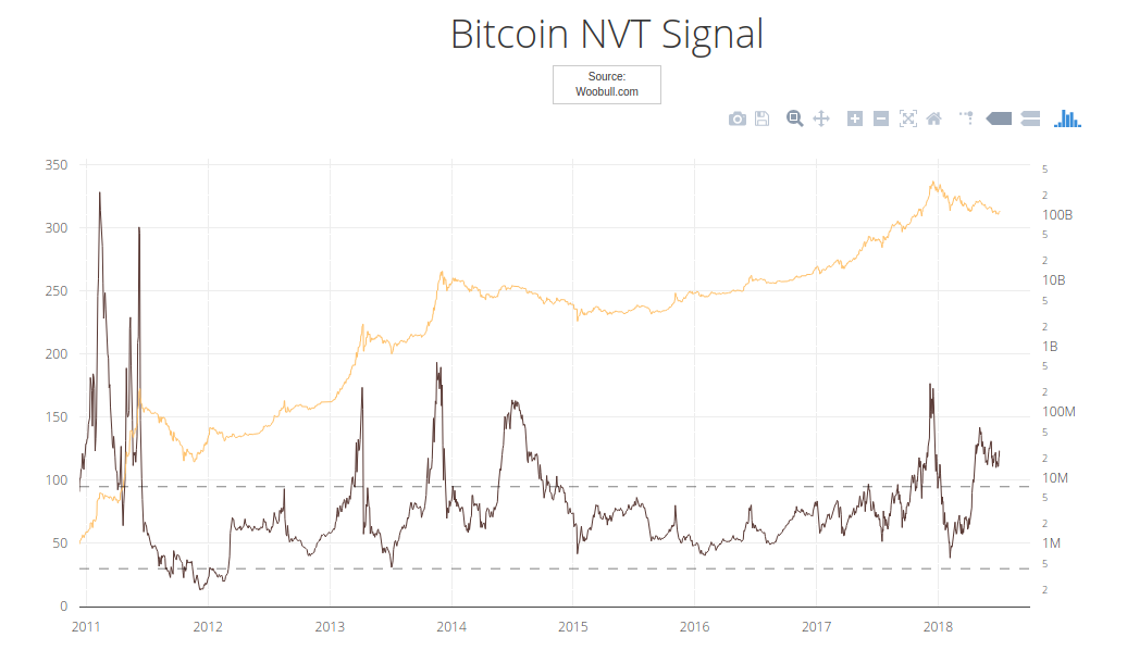
In Woobull Charts site we can inspect Bitcoin $NVT_{ratio}$ and Bitcoin $NVT_{signal}$ over time. In the following chart, the orange curve represents the Bitcoin market capitalization over time in logartithmic scale, and the black curve represents the $NVT_{signal}$. We can see how overvalued periods with high $NVT_{signal}$ are followed by bitcoin falling prices.
We can also calculate the $NVT$ ratio for different blockchains to obtain a relative valuation between them. Getting yesterdays’s (2nd July 2018) data from coinmetrics we can make simple calculations to compare some cryptoassets:
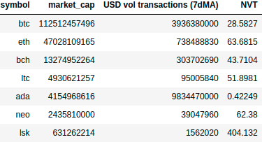
I’ve used 7 day moving average on dollar volume of daily transactions to filter oscillations. Currently, Cardano $NVT$ ratio is too low compared with other major cryptoassets, which means that the network is highly demanded. That’s a bullish signal. On the other hand, Lisk $NVT$ ratio is the highest, which could be interpreted as bearish.
Metcalfe’s Law
Metcalfe’s law was initially used for telecommunication networks and stated that the value of the network is proportional to the square of the number of connected users of the system:
\begin{equation}
net \propto (U)^2
\end{equation}
where $net$ is the network value and $U$ is the amount of users. It has been shown that social media networks seems to follow Metcalfe’s law. In Digital Blockhain Networks Appear to be Following Metcalfe’s Law, Dr. Ken Alabi showed that blockchain networks also behave the same way. Using Daily Active Address (DAA) as the number of connected users of the system per day, and market capitalization as the value of the network, we can compute Metcalfe’s ratio (MET) as:
\begin{equation}
MET = \frac{M}{(DAA)^2}
\end{equation}
where $M$ is the market capitalization of the cryptoasset and $DAA$ are the Daily Active Users. Metcalfe’s law is useful to analyze the network value growth as a function of connected users. This analysis is complex, and we will do it in a later article. Here only an introduction to the use of Metcalfe’s law was presented. Also, we are going to study a variation to the Metcalfe’s law, the Odlyzko law.
We can also try to compare $MET$ values between different blockchains. Taking yesterday’s data (2nd July 2018) from coinmetrics, let’s make some quick calculations:
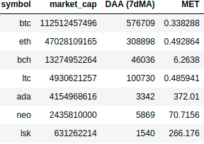
I’ve used 7 day moving average on daily active users to filter oscilations. In this case, Cardano and Lisk Metcalfe’s ratios are too high compared to other blockchains, which is related to the small number of users making transactions.
Absolute Valuation Methods
Now let’s try to find some intrinsic value to the cryptoassets. In this section we review:
- Cost of production model
- INET model
- VOLT model
- Discount Cash Flow model
Cost of Production Model
This model applies to crytocurrencies which could be mined, like Bitcoin. We try to estimate what is the cost that miners have generating coins. Assuming that miners are not willing to sell that coins at lower prices (otherwise, they would never have mined because the business would not be profitable), this value give us a fundamental value to the cryptocurrency.
Let’s try to find out the actual cost of production of 1 bitcoin (BTC). Electricity cost varies along the world, so we can use different values to estimate different costs of production. Supposing miners are using the Antminer S9 we can estimate the computation hashrate and the power that it consumes. You can play with values in the following python code to estimate the cost of production of 1 BTC:
import numpy as np

countries = ["Georgia", "China", "EEUU"]
electricity_cost = np.array([0.05, 0.08, 0.12]) # USD/KWh
hash_rate = 12930*10**9 # H/s (Antminer S9)
power_use = 1.375 # KW
difficulty = 5*10**12

time_to_find_a_block = difficulty*2**32/(hash_rate) # take a look at https://en.bitcoin.it/wiki/Difficulty
reward_per_block = 12.5
BTC_mined_per_sec = reward_per_block / time_to_find_a_block

secs_per_hour = 3600
electricity_cost_per_sec = power_use/secs_per_hour*electricity_cost
cost_to_produce_1_btc = electricity_cost_per_sec / BTC_mined_per_sec

print("Country", "BTC Cost [USD]")
for country, cost in zip(countries, cost_to_produce_1_btc):
    print("%s\t%.2f"%(country, cost))
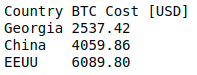
At the current difficulty, the cost of production of 1 BTC in EEUU is \$6089.8. Note that this model is dynamic: if prices drop, there could be less miners connected to the blockchain, the difficulty could decrease and so the cost of production. Some model improvements could include mining hardware costs, which are not covered here. In this case you would need to use a Discounted Cash Flow model.
INET Model
My favorite model used in cryptoasset valuations is the INET model developed by Chris Burniske. This model is useful for coins (or cryptocurrencies) and mostly for utility tokens, but it can’t be used to valuate security tokens. The main idea is to characterize the market in which the currency is going to be used. For example, FileCoin is used to pay for services in the cloud storage market, and FunFair is used in online gambling market. Making an idea of the Total Addressable Market (TAM) and the market the cryptoasset could efficiently absorb (let’s say, a 1% or a 5% or the TAM), we can estimate the size of the monetary base necessary to support a cryptoeconomy. Comparing that monetary base with current market capitalization, we can analyze if prices are over or undervalued. The model has several steps and some assumptions are requirements. Let’s build a model for a cryptoasset, in order to review what considerations should we make at each step.
I propose to build the model for Stellar. I choose Stellar because I haven’t seen any valuation model about this cryptoasset yet (it doesn’t mean there couldn’t be any one out there, I just couldn’t found it). Stellar is an open-source payment technology and its native coin is called lumen (XLM). XLM price has shooted up an incredible 41900 \% in 2017 and was one of the last year’s star performers. Is that growth justified? Let’s try to find out. You can follow all the ideas we’re going to comment below in this spreadsheet.
Total Addressable Market (TAM)
First at all, we have to make some research to characterize the TAM of the cryptoasset. Stellar network use cases are:
- Remittances
- Mobile branches
- Mobile money
- Micropayments
- Services for the underbanked
Making some internet research we get some numbers: from Transparency Market Research we estimate a 492 billion dollar TAM in 2017, with a forecasted Composed Annual Growth Rate (CAGR) of 20% until 2024, for the mobile payments market. This TAM includes most of the markets displayed above. It’s difficult to estimate a different TAM for each one, since the frontiers between them are diffuse. Besides, it’s not necessary, we can work with a global number. Another market in which Stellar could compete is the ICOs market, since the network allows dApps development. The first major token built on Stellar is Mobius, with a 15 million dollar market capitalization, and this is just the beginning (see stellar.org/blog/using-stellar-for-ico/ for more details on using Stellar as an ICO platform). In 2017 ICO funding surpassed 5 billion dollars and just in first quarter 2018 it has passed this value. We don’t have enough data to forecast this market, so we can’t characterize it well. I propose that we estimate another 20% CAGR for the ICO funding just for mathematics simplifications (I think we are being conservatives with this). The error of this approximation can’t be significant because the ICO funding market is much lower than the mobile payments market (5 billions to 492 billions).
Adoption Curve
Second, we have to estimate the adoption curve. The mobile payment market is a highly competitive market with companies like Visa, Paypal, Google, Apple and Microsoft, so it’s really difficult to shoot a guess here. We can create three different scenarios: a bullish scenario in which Stellar success reaching the 20% of the TAM in the long term, a moderate scenario in which Stellar absorbs the 10% of the TAM and a bearish scenario in which Stellar only keeps the 1% of the TAM.
It has been shown that innovative adoption follows an S curve. In order to fit the curve, we need to define a year in which starts the fast growth of adoption, and how long will it take for Stellar to go from 10% to 90% of saturation percentage of the TAM. Again, these are going to be assumptions and so we can play with different scenarios.
Network Dynamics
Next, let’s model the coin network dynamics. It would be good to know:
- how many coins are going to be held each year by Stellar foundation
- how many coins are going to be held by investors or stake holders
- if there is a projected inflation/deflation
- how fast the coins could go hand in hand
In Stellar dashboard we can follow the lumens distribution progress:
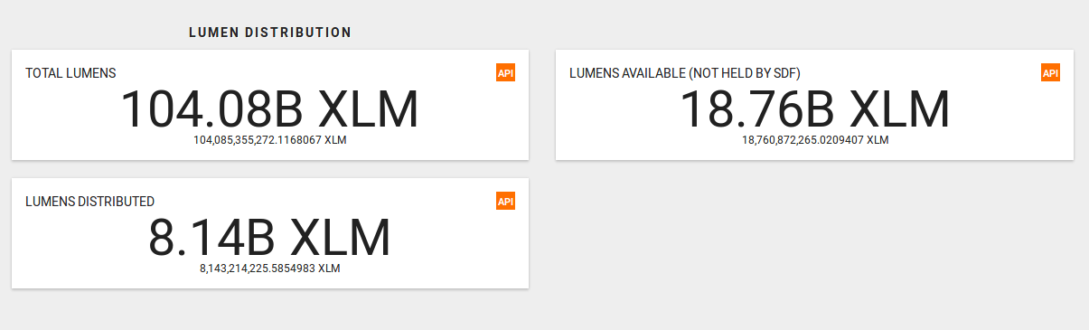
Currently, less than the 10% of total lumens has been distributed, and the rest are held by Stellar Development Foundation (SDF). In Stellar Development Foundation Mandate SDF clarifies that 95 billion lumens are going to be distributed to the world. They don’t give any specifications about how this distribution is going to be carried out, despite the fact that they (and Stripe, an early investor) are compromised to held this coins at least for 5 years since 2014, i.e., at least until 2019, in order to provide market stability to lumens. But what will happen next? I suggest to be conservatives here, and make the calculations assuming that all tokens are available in the economy. I said conservatives, because for a given economy, if we increase the amounts of coins, each coin tends to suffer devaluation (see the equation of exchange below).
What about inflation? New lumens are added to the network at the rate of 1% each year. Stellar distributes this lumens according to a voting system: each account votes for another account as its inflation destination, and this vote is weighted by the lumens held. Any account that gets over .05% of the votes from other accounts in the network receives part of this new coins, and also a part of the Fee Pool (all the collected fees in a given period). However, considering that fees in Stellar network are excessively low, it seems that Fee Pool distribution is unlikely to be a significant contributor to XLM token holder returns.
Given the above discussion, it’s hard to estimate what percentage will be staked. Some cryptos using PoS as consensus algorithm have over 50% supply staked, like PIVX. Stellar doesn’t use PoS, (it uses a Federated Bizantine Agreement), but it could helps as a starting point. Let’s assume a 50% staking ratio.
Money Velocity
The last thing we have to model is the velocity of the money: the frequency at which one unit of currency is used to make a payment. This is related with how fast the coins could go hand in hand. The greatest the velocity, faster the money passes from one holder to the next. To figure out how an Stellar economy with a high velocity would be, let’s make an example: If I want to pay you using the Stellar network, I would have to purchase some lumens on an exchange because the last lumens I get paid I sold immediately, afraid of being devalued. So, once I get some lumens again, I make you the transaction. You receive your lumens and quickly sell them to some one else, this time not because of fear of devaluation, but simply because you do not give them any use. In this kind of economy, coins are going to suffer devaluation compared to an economy in which participants have incentives to retain the coins, i.e., with lower velocity. There are some mechanisms to reduce velocity, but we are not going to discuss them here. To have some points of comparison:
- USD M1 money stock velocity is 5.5 (M1 refers to currency in circulation).
- Bitcoin circulating coins velocity was approximately 14 in 2016 according on Chris Burniske calculations based on a research he did with Coinbase on how their users interact with bitcoin.
Since Stellar lumens are currencies and not tokens used to purchase specific services, I think that we can also assume the same velocity than bitcoin, thinking in a mid-long term. In the short term velocity could be greater due to speculation. This is the strongest assumption we have to make in the model. In the VOLT section we are going to see an alternative way to model this parameter.
Equation of Exchange
Now, in order to put all together, we have to talk about the equation of exchange. This equation showcases the relationship between all things we have been discussing so far in the INET section. The equation stands that:
\begin{equation}
M \cdot V = P \cdot Q
\end{equation}
where $M$ is the average nominal amount of money supply in circulation in a given period, $V$ is the velocity of the money in that period, $P$ is the average price level of goods in that period and $Q$ is the index of expenditures also in that period. A cryptoasset valuation is largely comprised of solving for $M$, where $M = P\cdot Q / V$. $M$ is the size of the monetary base necessary to support a cryptoeconomy of size $PQ$, at velocity $V$. It’s important to clarify that $P$ does not represent the price of the cryptoasset. It represent’s the price of the resource being provisioned by the cryptonetwork, like average online game prices in FunFair. $Q$ represents the quantity of that resource provisioned, like the amount of online games payed. In the case of Bitcoin and Stellar, where their native currencies are used for payments, $P\cdot Q$ is related with the estimated transaction value in the network. If we consider the equation in annual terms, we can relate $P\cdot Q$ with the absorbed market we’ve been discussing previously.
And what about $M$? $M$ stands for the money supply necessary to maintain an economy with $V$, $P$ and $Q$. So it represents the market capitalization of the circulating currencies:
\begin{equation}
M= P_{xlm} \cdot N_{xlm, circulating}
\end{equation}
where $P_{xlm}$ is the utility price of each coin and $N_{xlm, circulating}$ are the total amount of circulating coins.
Speculative Value
According to Chris Burniske analysis in this another great article, cryptoasset’s price is composed of two forms of value: “current utility value” (CUV) and “discounted expected utility value (DEUV)”, the last best known as speculative value. Speculative value is related with how much a participant who purchases some coins today expects to earn holding this asset for a given period of time. Based on forecasted prices using the exchange equation, investors can assign a present value to the currencies according to the discount rate they are willing to assume, given the risk of the investment. Which discount rate would we use in order to calculate present value of future prices? What we can do here, is try to compare this investments with venture investments, since this is a field that has a lot of study. According to Prof. Aswath Damodaran from the New York University, a recognized figure in the field of young companies valuations, the target rates of return demanded by venture capitalists, are categorized by how far along a firm is in the life cycle:
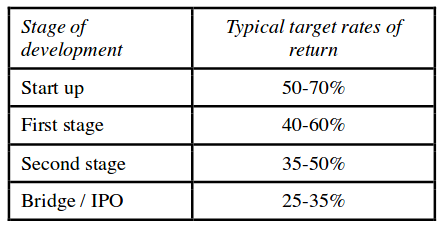
Since Stellar has completed its early stages I think investors are willing to accept discount rates between $30\$%$-$40\%$. This is purely subjective and you can play with this number later.
Simulation
Putting all together in the spreadsheet, we have to make one last assumption in order to forecast the simulation beyond 2024. We have not data about market growth, so the best is to be conservatives and estimate that the growth stops being so pronounced. Let me forecast our data using an exponential CAGR decrease.
Now, let’s see the results using our first bullish scenario, where Stellar adopts $20\%$ of TAM in the long term, with start of fast growing adoption in three years and five more years to hits 90% of market saturation. The following curves show market adoption and the network transaction value:
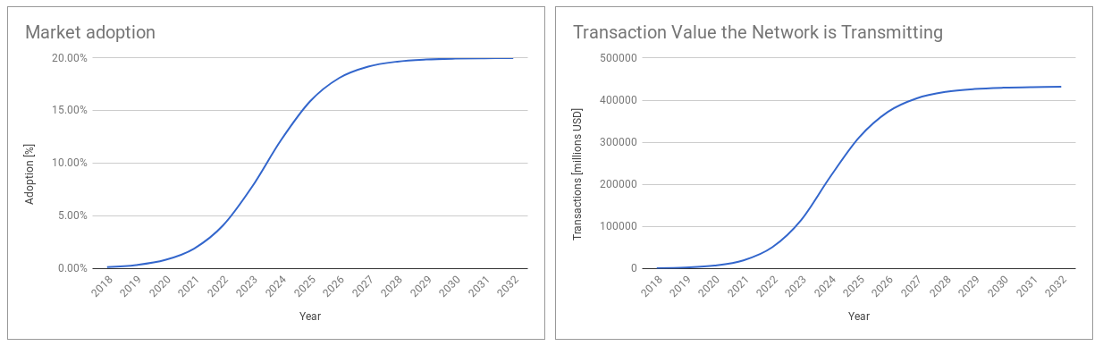
Supposing $50\%$ of lumens held by investors, in the following charts we see how much circulating coins will be each year and coin prices predicted by our model:
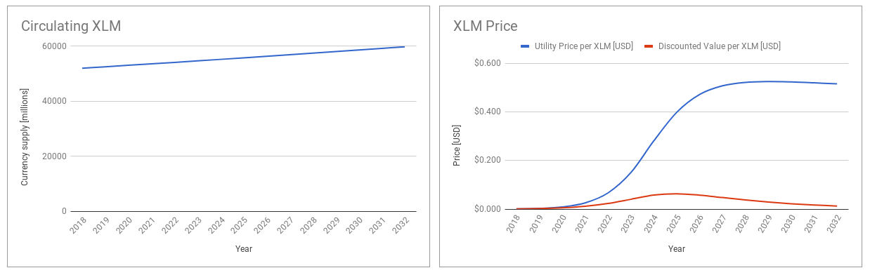
The chart on the left simply shows that circulating lumens are incremented each year due to inflation. On the right, the blue curve models the utility price per year, per lumen. Acording to the adoption curve we’ve defined, values are lower at the beginning due to the limited use, and grow following the usability. In the long term, once the market has been adopted, they experiment a little decrease due to inflation (but remember we don’t have data about how the mobile payment market will continue). The red curve models the discounted value of future prices for each year, assuming a discount rate of $30\%$. We find the maximum on that curve in 2025 at $\$0.064$, which could be read as following: Investors who consider the previous scenario, today are willing to pay a maximum of $\$0.064$ per lumen, expecting a $30\%$ return on investment per year until 2025.
What happens if we analyze a moderate scenario (market saturation: 10%, year of fast growth: 2021, time to hits 90% of saturation: five years) and another bearish one (market saturation: 1%, year of fast growth: 2021, time to hits 90% of saturation: seven years)?
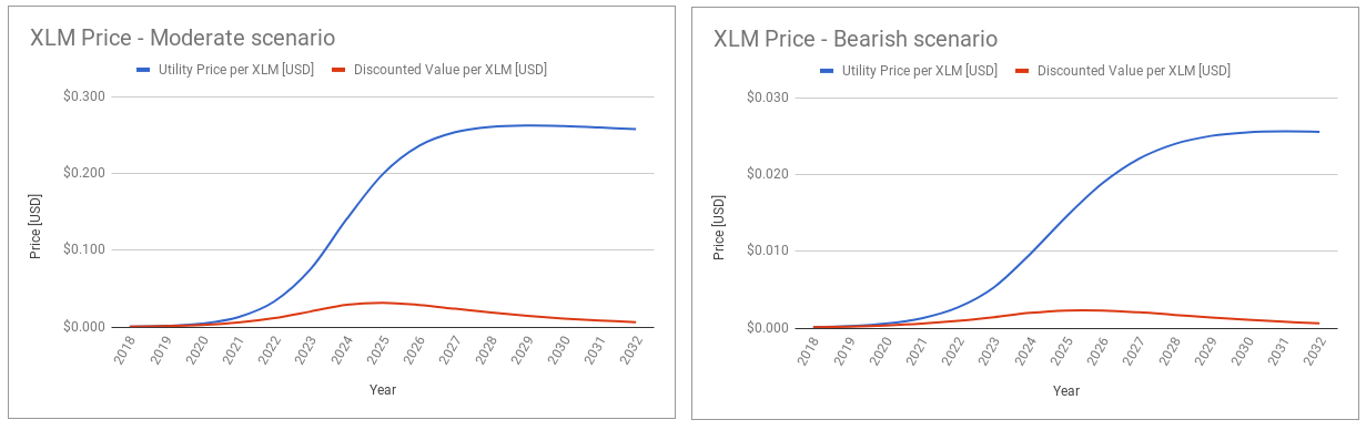
Well, in the moderate scenario the maximum lumen discounted value is $\$0.032$ and in the bearish scenario $\$0.002$. At market rates around $\$0.20$, we conclude that currently lumens are overvalued. However, we should consider that we have been making a lot of assumptions. I recommend you to play with parameters and forecast your own results using the spreadsheet.
VOLT Model
In the previous model, we’ve assumed a fixed value to the velocity of the money, which was arbitrary. Alex Evans from placeholdervc has proposed a framework to model the velocity using the Baumol-Tobin model. The Baumol-Tobin model relates the transactions demand for money with the transaction costs and interest rate of risk-free investments. The basic question it tries to solve is the following: Suppose I am a participant in a given economy in which I have a monthly income P and I spend all that money during month. I can choose between
- holding P in cash liquid all month
- making a deposit of P in an interest bearing bank and then make partial withdrawals each time I need.
The last choice makes me earn some money from investments, but also makes me spend a lot of money due to transaction costs. I suspect the optimal choice should be in some point between them. So, which is the optimal number of withdrawals should I do in order to maximize my earnings (or minimize my forgone returns)?
Modeling the transaction costs on the network, and relating the risk-free investments with some store of value asset, we can predict the optimal amount of transactions will do each participant in the network. From that, we can calculate the velocity of the money as:
\begin{equation}
V=\sqrt{\frac{2\cdot R \cdot Y} {C}}
\end{equation}
where $R$ is the risk-free nominal interest rate, $Y$ are the average payments per user per year and $C$ is the cost per transaction. All this parameters depends on time and so we get a dynamic model for the velocity.
Discount Cash Flow (DCF) Model
I left to the end the quantitative valuation model commonly used to analyze stocks and startups, which could help us as a framework to valuate security tokens. Security tokens are cryptoassets subjected to federal securities regulations, and derives their values from external assets. The reason for the contributors to buy the tokens, is the anticipation of future profits in form of dividends, revenue share or price appreciation. This is why I think that a Discounted Cash Flow analysis fits perfect here.
DCF is a valuation method used to estimate the attractiveness of an investment opportunity. Iit is based on the idea of time value of money, which stands that money has greater value now than later. DCF analysis use future free cash flow projections and discounts them, using a required annual rate, to arrive at present value estimates. We can compare the present value with the investment value to decide if it’s a good investment or not.
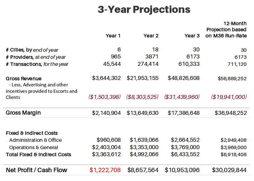
The first step to perform the DCF analysis is to analyze the cash flow of the project. Which project can we analyze? So far there have been few projects created with security tokens, and I have found only one that presents a forecasting cash flow. That project is Pinkdate, the Escorting Platform. Pinkdate’s whitepaper presents the following cash flow projection:
The next step is to estimate a Terminal Value (TV) for the project. TV can be approached using the Gordon Growth model:
\begin{equation}
TV = \frac {CF_{final} \cdot (1 +GR)}{(d_r -GR)}
\end{equation}
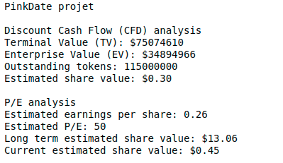
where $CF_{final}$ is the final project year cash flow, $GR$ is the long term cash flow growth rate and $d_r$ is the discount rate. The estimated final project year cash flow is 30 million dollars. Supposing a zero long term cash flow growth rate and a $40\%$ discount rate we calculate a \$75 million dollar TV.
To complete the analysis, we need to compute the discounted sum, in order to estimate an Enterprise Value (EV):
\begin{equation}
EV = \sum_{i=1} ^{i=3} \frac{CF_i}{{(1+r)}^i} + \frac{TV}{{(1+r)}^3} \approx \$35 \:millions
\end{equation}
With 115 million outstanding tokens, each token value should be something around \$0.3. That means that investors in the pre-iCO stage which payed between \$0.14 and \$0.17 have made a good investment, but according to this model, the ICO \$0.588 value is overvalued.
We can also try another interesting analysis. In the long term, the earnings per share price will be approximately \$0.26 (30 million dollar long term cash flow divided by the amount of outstanding tokens). Based on a tech/startup P/E of 50, the reference per share price could be \$13 (\$50 · \$0.26). If this cash flow is reached in 8-10 years, the present value per share is something between \$0.45 and \$0.88.
You can play with the following code to analyze the parameter sensitivity to the previous discussion:
print("PinkDate projet")

print("\nDiscount Cash Flow (CFD) analysis")
tokens = 115*10**6
cash_flow=[-1222708, 8657564, 10953096]
final_project_year_cash_flow = 30029844
long_term_cash_flow_growth_rate = 0
discount_rate = 0.4
TV = final_project_year_cash_flow * (1+long_term_cash_flow_growth_rate) / (discount_rate - long_term_cash_flow_growth_rate)
EV = 0
for i, cf in enumerate(cash_flow):
    EV += cf/(1+discount_rate)**(1+i)
EV += TV/(1+discount_rate)**3
print("Terminal Value (TV): $%d"%TV)
print("Enterprise Value (EV): $%d"%EV)
print("Outstanding tokens: %d"%tokens)
print("Estimated share value: $%.2f"%(EV/tokens))

print("\nP/E analysis")
estimated_price_per_earnigs = 50
long_term_years = 10
estimated_earnings_per_share = final_project_year_cash_flow/tokens
long_term_estimated_price = estimated_earnings_per_share * estimated_price_per_earnigs
current_estimated_price = long_term_estimated_price/(1+discount_rate)**long_term_years
print("Estimated earnings per share: %.2f"%estimated_earnings_per_share)
print("Estimated P/E: %d"%estimated_price_per_earnigs)
print("Long term estimated share value: $%.2f"%long_term_estimated_price)
print("Current estimated share value: $%.2f"%current_estimated_price)
Multicoin Capital has made a similar interesting analysis on Augur REP tokens using the discount cash flow model. Augur is a decentralized prediction market, and REP holders are entitled to reporting fees (in this case, this are not dividends paid from security tokens, but we can take them as if they were). Estimating a $25 billion dollar market generated from total reports, at a 1\% reporting fees rate, the annual return per REP is approximately \$22.73 per token (25 billion dollars multiplied by 1% and divided by 11 million tokens). Again, considering a 50 P/E ratio, REP tokens will be trading at \$1136.5. Now we have to discount this value from the year it will be reached (let’s say, in 3-5 years) to 2018. Using a 40% discount rate we have a present value between \$211 and \$414. Since REP tokens are currently being trading at approximately \$36, this model concludes they are undervalued.
Final Words
In this article we have being reviewing some of the most useful cryptoasset valuation frameworks I have found. It’s important to note that all the calculations we have made were made for educational purposes only. Before using some model to valuate a cryptoasset and decide on your investments, I recommend you to deeply research the project and to analyze parameter sensitivity in different scenarios. Each example should be interpreted as a framework to start and not as final valuation.
If you liked this article, you might also like:
- Value at Risk & Expected Shortfall of Cryptocurrencies
- Cryptocurrency Investment Spreadsheet
- Emerging New Trends in Blockchain Technologies
- What I Have Learned From My Arbitrage Experiences with cryptoassets
Disclaimer: CoinFabrik does not provide financial advice. This material has been prepared for educational purposes only, and is not intended to provide, and should not be relied on for, financial advice. Consult your own financial advisors before engaging in any investment.